Advanced Macro Seminar
Machine Learning for Economics Research
Ching-Yang Lin
2026-05-12
Can We Use Machine Learning for Economics?
Machine learning is everywhere — recommendation systems, self-driving cars, language models.
But can we use it for economics research?
If it’s so powerful, why don’t we see it more in economics journals? Why doesn’t our econometrics curriculum cover it?
Two Obstacles (and Why They’re Shrinking)
1. Data volume
Traditional econometrics works with small, carefully collected datasets. ML needs large samples. But survey data is getting bigger (SCF: 55,000 households), administrative data is exploding, and text data is now usable.
2. Causality
Econometrics asks why — the causal effect of X on Y. ML asks what — the best prediction of Y from everything available.
But the gap is closing. Double/Debiased ML, Causal Forests, and SHAP decomposition are bridging prediction and causal inference.
This Course: Three Components
Component 1: What is ML and what does a research workflow look like?
The main algorithms, the process from data to evaluation to interpretation.
Component 2: How do we actually do it?
Modern AI coding assistants (Claude Code, Codex) let you build ML pipelines by describing what you want in natural language. Live demo today.
Component 3: Can ML handle causality?
Yes, increasingly. Methods that combine ML’s predictive power with the causal reasoning economists care about.
Part 1
Why Machine Learning?
What is Machine Learning?
A set of methods that learn patterns from data instead of being explicitly programmed.
Traditional programming:
Rules + Data → Output
Machine learning:
Data + Output → Rules (learned automatically)
The computer figures out the rules by seeing examples.
A Simple Example
Predicting whether a student passes an exam:
| Study Hours | Attendance | Pass? |
|---|---|---|
| 10 | 90% | Yes |
| 2 | 40% | No |
| 8 | 85% | Yes |
| 3 | 50% | No |
| ??? | ??? | ??? |
You can probably see the pattern. ML algorithms do this automatically, even with hundreds of variables.
Types of Learning
Supervised Learning (today’s focus)
- We have a target we want to predict
- The algorithm learns from labeled examples
- Classification: predict a category
- Regression: predict a number
Unsupervised Learning
- No target variable
- Find hidden structure in data
- Clustering, dimensionality reduction
- Not covered today
AI Systems You Already Use — Which Type?
| System | What It Does | Learning Type |
|---|---|---|
| YouTube recommendations | Predicts which video you’ll click next | Supervised |
| Instagram / TikTok feed | Predicts which posts you’ll engage with | Supervised |
| Amazon “customers also bought” | Predicts what you’ll purchase | Supervised + Unsupervised |
| Email spam filter | Classifies email as spam or not | Supervised (classification) |
AI Systems (continued)
| System | What It Does | Learning Type |
|---|---|---|
| Self-driving cars | Detects objects, predicts trajectories | Supervised + Reinforcement |
| AlphaGo / chess engines | Learns winning strategies by playing | Reinforcement Learning |
| ChatGPT / Claude / Gemini | Predicts the next token in a sequence | Self-supervised* |
*LLMs are trained on massive text without explicit labels — the “label” is the next word itself.
The Key Distinction
Supervised: Someone tells the model the right answer during training.
- “This email IS spam” / “This email is NOT spam”
- “This household holds stocks” / “This household does not”
Unsupervised: No right answers — the model finds structure on its own.
- “Group these customers into segments” (clustering)
Reinforcement: Learn by trial and error (rewards / penalties).
- AlphaGo: win = reward, lose = penalty
Today we focus on supervised learning.
Classification vs Regression
| Classification | Regression | |
|---|---|---|
| Target | Category (Yes/No, A/B/C) | Number (price, score) |
| Example | Does this person own stocks? | How much do they invest? |
| Output | Probability + label | Continuous value |
| Metrics | Accuracy, AUC, F1 | RMSE, R² |
Today: classification — predicting stock market participation.
Why ML in Economics?
Traditional econometrics asks: “What is the causal effect of X on Y?”
Machine learning asks: “Can we predict Y from all available information?”
These are different questions, and both are useful.
| Econometrics | Machine Learning | |
|---|---|---|
| Goal | Causal effect of one variable | Best prediction using all variables |
| Variables | Few, carefully chosen | Many, let the data decide |
| Evaluation | Coefficient significance | Out-of-sample prediction accuracy |
Today’s Research Question
Can we predict who participates in the stock market?
- Data: Survey of Consumer Finances (SCF), US Federal Reserve
- 55,000 households, surveyed every 3 years (1992–2022)
- Rich information: income, wealth, education, risk attitudes, demographics
- Target: Does this household hold any stocks? (Yes/No)
This is a real research question from my own work.
The SCF Dataset at a Glance
| Feature | Type | Examples |
|---|---|---|
| Demographics | Categorical | Education, Marital Status, Work Status |
| Financial | Numerical | Income, Net Worth, Total Assets, Debt |
| Risk attitudes | Categorical | Risk Aversion level |
| Housing | Binary | Home Ownership |
| Macro conditions | Numerical | VIX, Stock Returns, Unemployment |
| Target | Binary | Has_Total_Stock (0 or 1) |
55,004 observations across 11 survey waves.
What We’ll Do Today
Part 1: Why Machine Learning?          <-- You are here
Part 2: The ML Process
Part 3: Live Demo with SCF Data
Part 4: Evaluation Deep Dive
Part 5: Model Comparison
Part 6: SHAP --- Understanding Predictions
By the end, you will have built a complete ML pipeline from scratch.
Part 2
The ML Process
The Workflow
1. Data  -->  2. Split  -->  3. Preprocess  -->  4. Train  -->  5. Evaluate  -->  6. Compare
                                  ^                                                   |
                                  |___________________ try another model _____________|
This workflow is the same regardless of which algorithm you use.
Master the process, and you can use any ML method.
Step 1: Get Your Data
- Understand what each variable means
- Check for missing values, outliers, data types
- Think about the problem before writing code
For SCF data:
- Why might someone participate in the stock market?
- Which variables would you use to predict this?
- Are there variables that would be “cheating”? (e.g.,
Total_Stock_Value)
Step 2: Split the Data
Before anything else, split into training and test sets.
- Training set (70%): used to build the model
- Test set (30%): locked away until the very end
Why? To simulate real-world performance — the model must predict on data it has never seen.
  Full Data (55,004 rows)
        |
   +---------+---------+
   |                   |
Training            Test
38,503 rows      16,501 rows
  (70%)            (30%)
Why Split FIRST?
A common mistake:
“I’ll preprocess all the data, then split.”
This is wrong. If you compute the mean of all data and use it to fill missing values, the test set has “seen” training data information.
This is called data leakage — your test results will be too optimistic.
Rule: Split first. Preprocess training and test sets separately.
(Pipelines handle this automatically.)
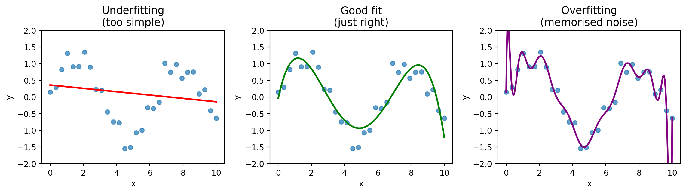
The Overfitting Problem
- Underfitting: model is too simple, misses the pattern
- Overfitting: model memorises noise, fails on new data
- Good fit: captures the pattern, generalises well
Cross-Validation
Problem: A single train/test split might be lucky or unlucky.
Solution: Repeat the process multiple times.
| Fold | Data Split |
|---|---|
| 1 | Train Train Train Train Test |
| 2 | Train Train Train Test Train |
| 3 | Train Train Test Train Train |
| 4 | Train Test Train Train Train |
| 5 | Test Train Train Train Train |
Each fold gets a score → report the average.
Step 3: Preprocess
Real data is messy. Common problems:
| Problem | Solution |
|---|---|
| Missing values | Impute (mean, median, or most frequent) |
| Different scales | Standardise (mean=0, std=1) |
| Categorical text | Encode (one-hot encoding) |
In scikit-learn, we handle this with Pipeline and ColumnTransformer — we’ll see the code in Part 3.
Step 4: Train a Model
Plug in any algorithm:
- Logistic Regression (simple, interpretable)
- Random Forest (ensemble of decision trees)
- Gradient Boosting (powerful, widely used)
- Support Vector Machine
- Neural Network
- …
The beauty of scikit-learn’s Pipeline: swap the algorithm in one line.
Algorithm Intuitions: Logistic Regression
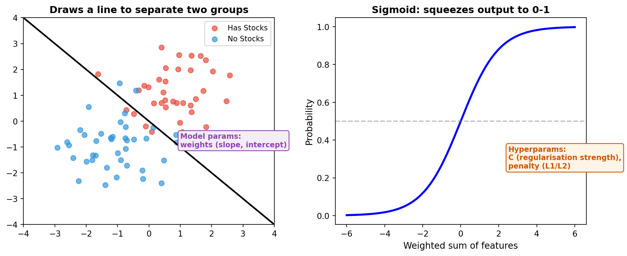
| Learned from data | Set before training | |
|---|---|---|
| Model parameters | Weights (one per feature), intercept | |
| Hyperparameters | C (regularisation), penalty type |
Algorithm Intuitions: Decision Tree
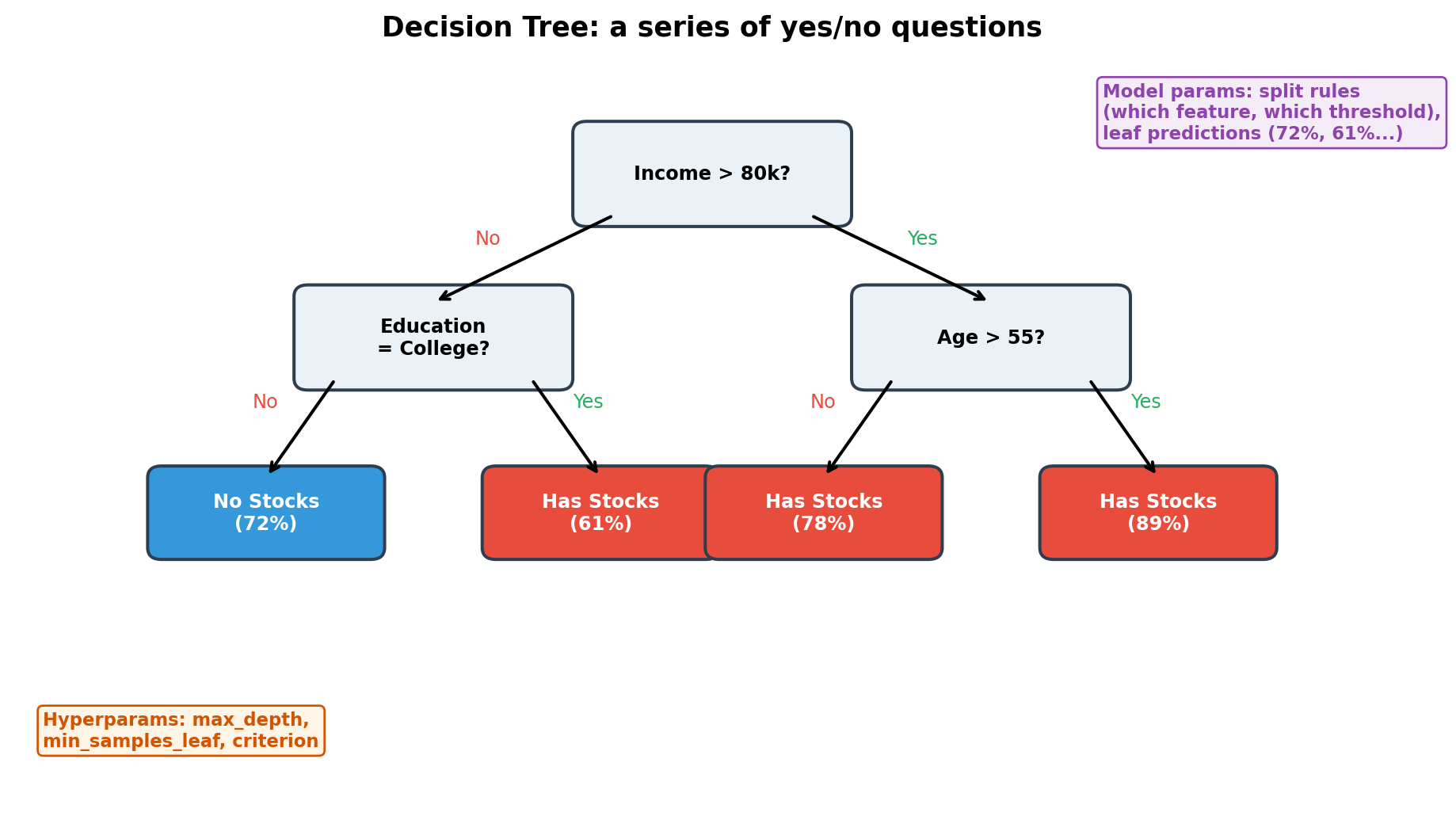
Easy to visualise and explain, but tends to overfit — memorises the training data.
Algorithm Intuitions: Random Forest
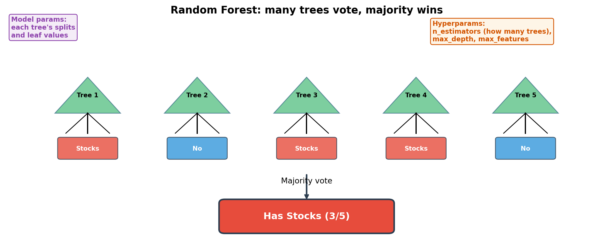
Build hundreds of trees on random subsets. Errors cancel out → robust ensemble.
Algorithm Intuitions: Gradient Boosting
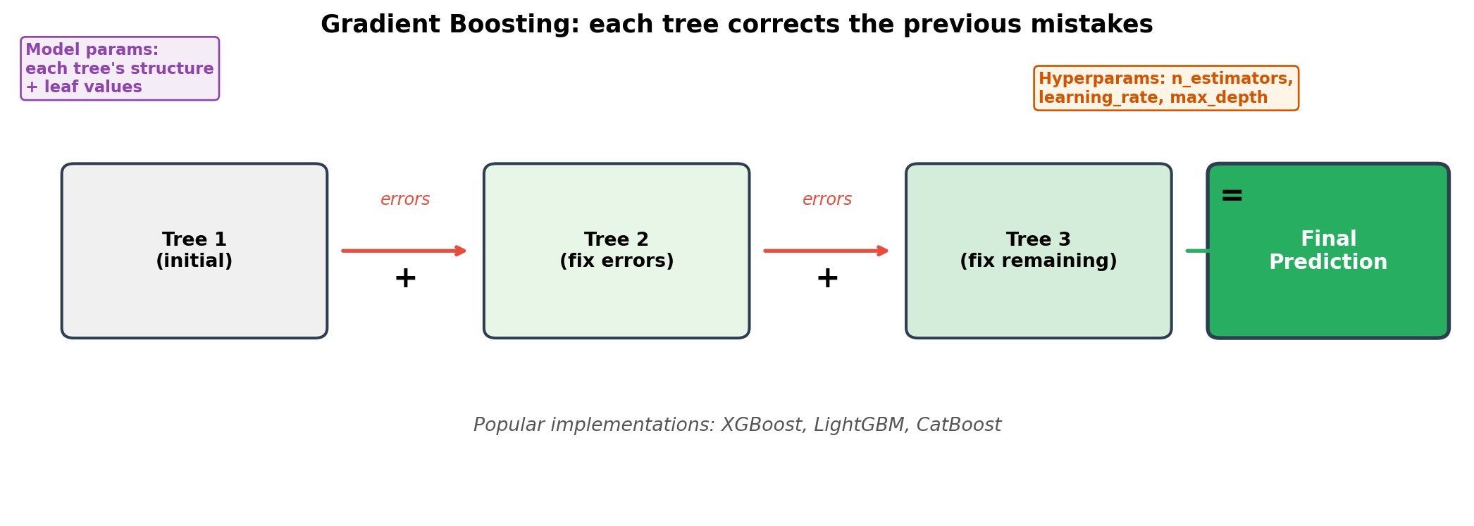
Sequential error-correction. Often achieves the highest accuracy, but slower to train.
Algorithm Intuitions: SVM
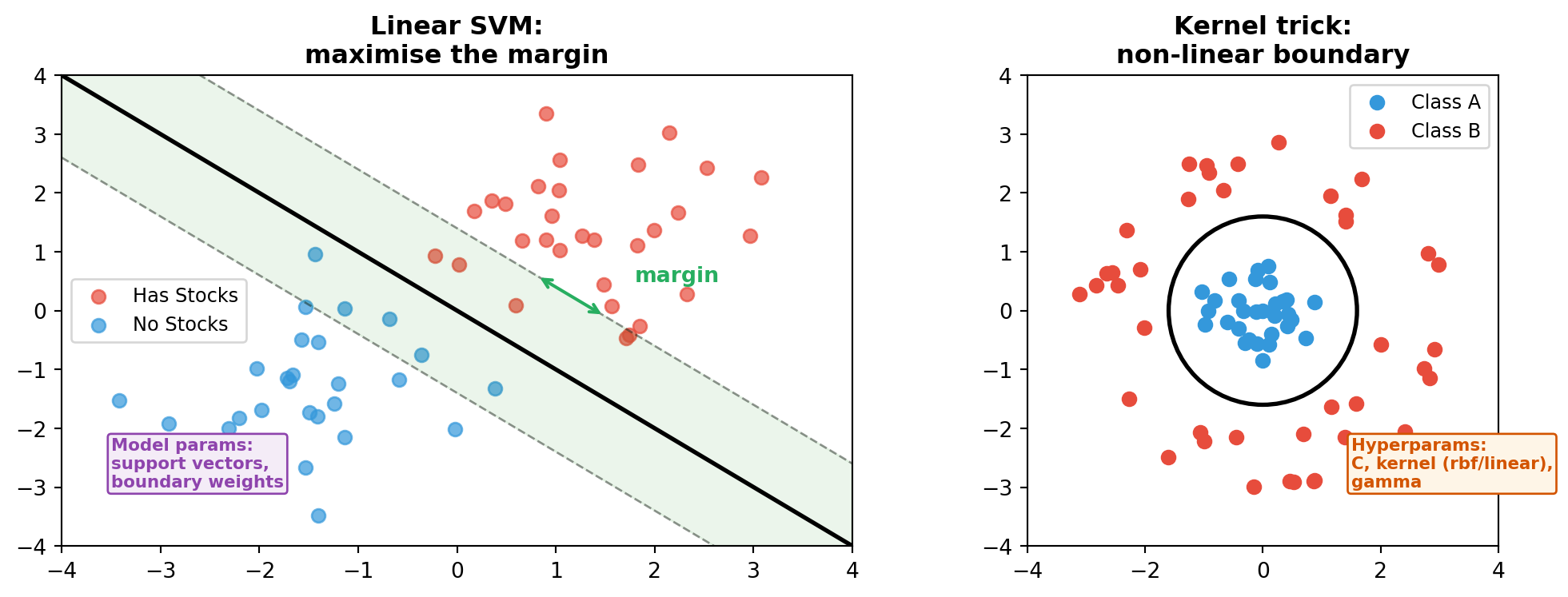
Finds the boundary with the widest margin. The kernel trick handles non-linear cases.
Algorithm Intuitions: Neural Network
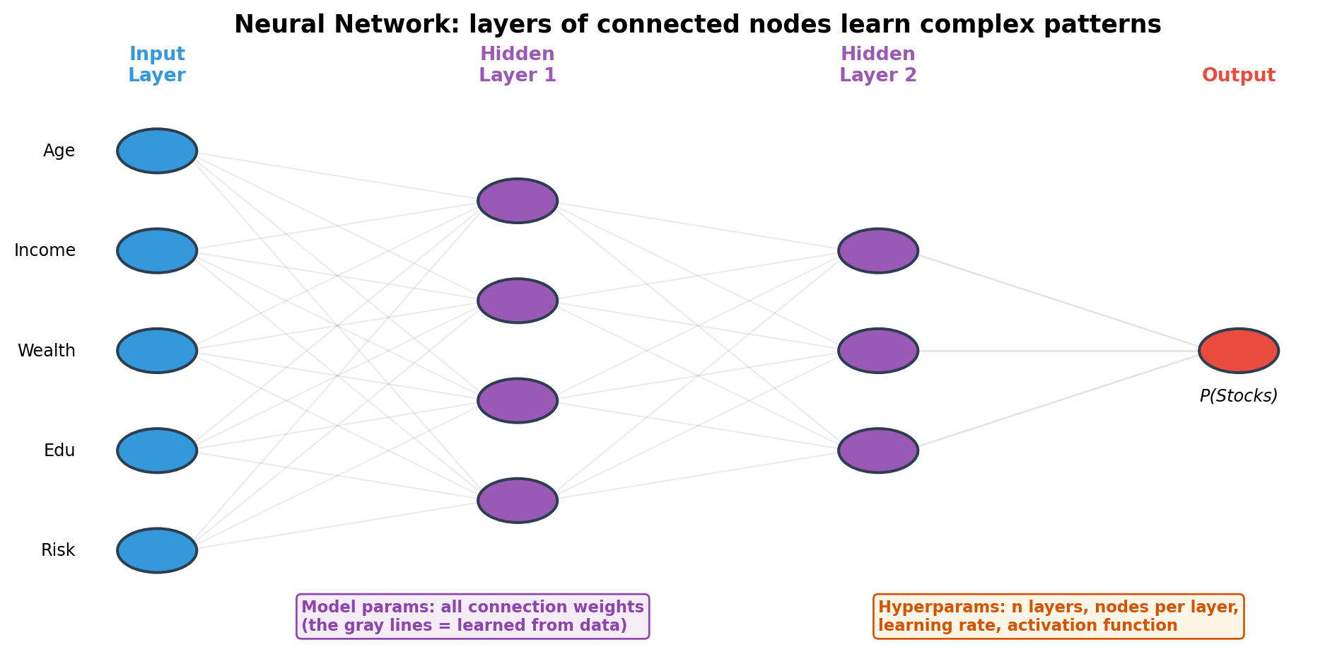
Each node: inputs × weights → activation function. Stacking layers = increasingly abstract features. LLMs (GPT, Claude, Gemini) are built on this architecture.
Unsupervised Learning: Clustering
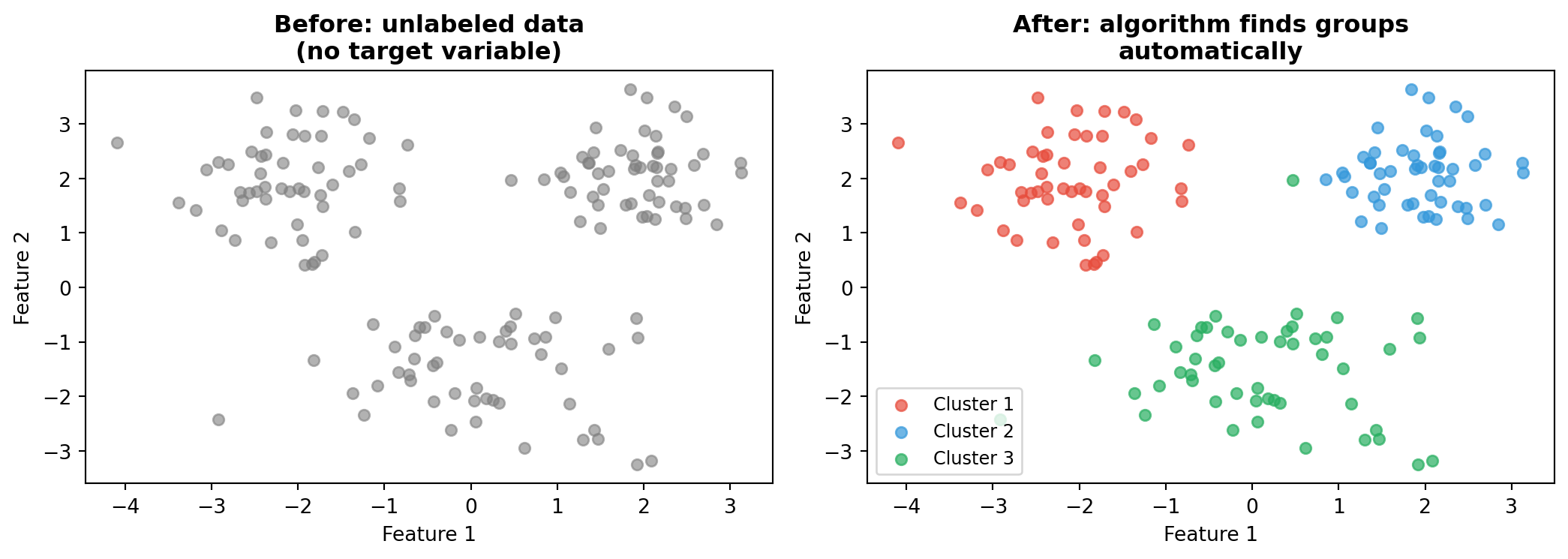
No labels needed. The algorithm discovers structure — e.g., customer segments, country groups, household types.
Unsupervised Learning: Dimensionality Reduction (PCA)
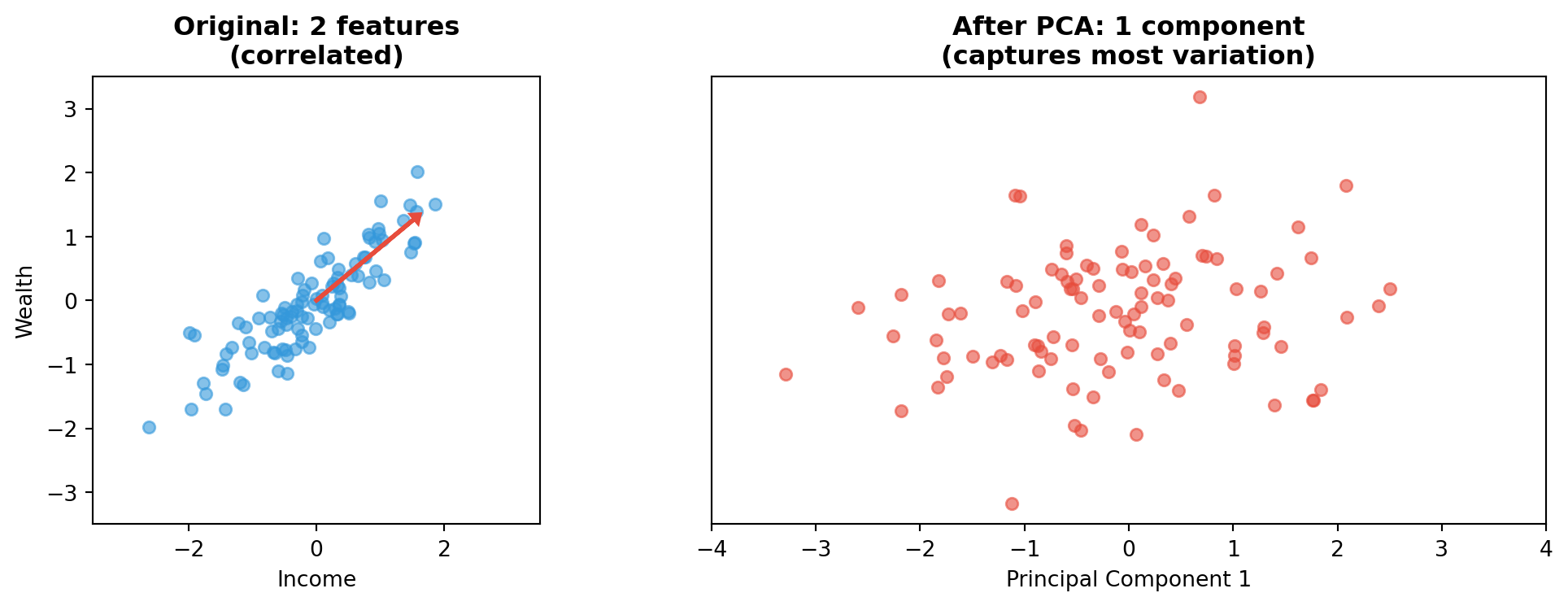
Reduces many features to a few key dimensions — useful for visualisation and noise removal.
The ML Library Landscape
| Library | Type | Use For |
|---|---|---|
| scikit-learn | Traditional ML | Logistic regression, trees, SVM, pipelines |
| XGBoost / LightGBM | Gradient boosting | High-accuracy tabular data models |
| PyTorch / TensorFlow | Deep learning | Neural networks, custom architectures |
All scikit-learn algorithms share a uniform .fit() / .predict() interface.
XGBoost/LightGBM are compatible with this interface too.
Model Parameters vs Hyperparameters: Summary
| Algorithm | Model Parameters (learned) | Hyperparameters (you set) |
|---|---|---|
| Logistic Regression | Weights, intercept | C, penalty |
| Decision Tree | Split feature, threshold, leaf values | max_depth, min_samples_leaf |
| Random Forest | All trees’ splits + leaf values | n_estimators, max_depth |
| Gradient Boosting | All trees’ structure + leaf values | n_estimators, learning_rate |
| SVM | Support vectors, boundary weights | C, kernel, gamma |
| Neural Network | All connection weights + biases | Layers, nodes, learning rate |
Model parameters: the algorithm finds these by optimising on training data.
Hyperparameters: you choose these before training. We use GridSearchCV to find the best combination.
Step 5: Evaluate
Never evaluate on training data!
Use the test set (held out since Step 2):
- Accuracy: what fraction did we get right?
- Precision, Recall, F1: more nuanced metrics
- ROC/AUC: overall ranking quality
We’ll dive deep in Part 4.
Step 6: Compare and Iterate
- Try multiple algorithms
- Compare their test performance
- Select the best one
Important: The process is the same every time. Only the model changes.
Part 3
Live Demo: Predicting Stock Market Participation
Coding with AI Assistants in 2026
We won’t just type code from scratch — we’ll use AI coding assistants to help us build the ML pipeline step by step.
Two categories of tools:
| Type | Examples | How It Works |
|---|---|---|
| Application (GUI) | Cursor, Codex (ChatGPT), Claude Desktop | IDE or chat interface, point-and-click |
| CLI (Terminal) | Claude Code, Codex CLI, OpenCode, Gemini CLI | Run directly in your terminal, works alongside your code |
Today we’ll use Claude Code in the terminal.
Setting Up the CLI Environment
| OS | Terminal | Extra Step |
|---|---|---|
| macOS | Terminal or iTerm2 | None |
| Windows | Windows Terminal | Install WSL first |
| Linux | Any terminal | None |
Install: npm install -g @anthropic-ai/claude-code
Run: claude in your project folder
What Can CLI AI Assistants Do?
In a CLI coding environment, the AI assistant can:
- Read your files — it understands your project structure
- Write and edit code — create scripts, fix bugs, refactor
- Run commands — execute Python, install packages, run tests
- Explain code — ask “what does this function do?”
- Iterate — “change the model to Random Forest” and it modifies the code
You describe what you want in natural language, and the assistant builds the code.
Demo: Building a Pipeline with Claude Code
Instead of copy-pasting code blocks, we’ll give instructions like:
“Load the SCF dataset from data/raw/SCF_with_Macro_and_Weights.csv. Show me the shape and the first few rows.”
“Build a scikit-learn pipeline with logistic regression. Use Age, Income, Net_Worth, Total_Fin_Asset, and Total_Debt as numerical features. Use Education, Work_Status, Marital_Status, Home_Ownership, and Risk_Aversion as categorical features.”
“Run 5-fold cross-validation with AUC scoring and show the results.”
The assistant writes the code, runs it, and shows you the output — all in the terminal.
Why Use AI Assistants for ML?
- Faster iteration — describe what you want, get working code
- Fewer syntax errors — the assistant handles boilerplate
- Learning tool — ask “why did you use StandardScaler here?” and get an explanation
- Focus on the process — you think about what to do, the assistant handles how to write it
The code below shows what the assistant would generate at each step. In class, we’ll build this live.
Setup
Code
# Import everything we need
import pandas as pd
import numpy as np
import matplotlib.pyplot as plt
from sklearn.model_selection import train_test_split, GridSearchCV, cross_val_score
from sklearn.preprocessing import StandardScaler, OneHotEncoder
from sklearn.impute import SimpleImputer
from sklearn.compose import ColumnTransformer
from sklearn.pipeline import Pipeline
from sklearn.linear_model import LogisticRegression
from sklearn.ensemble import GradientBoostingClassifier, RandomForestClassifier
from sklearn.metrics import (
    confusion_matrix, ConfusionMatrixDisplay,
    classification_report, roc_curve, auc,
    RocCurveDisplay, f1_score, accuracy_score
)
import warnings
warnings.filterwarnings('ignore')
Step 1: Load the Data
Expected output:
Dataset shape: (55004, 65)
Survey years: [1992, 1995, 1998, 2001, 2004, 2007, 2010, 2013, 2016, 2019, 2022]
Explore the Target Variable
Participation Over Time
Step 2: Select Features
Code
# Feature selection --- based on economic reasoning
numerical_features = ['Age', 'Income', 'Net_Worth', 'Total_Fin_Asset', 'Total_Debt']
categorical_features = ['Education', 'Work_Status', 'Marital_Status',
                        'Home_Ownership', 'Risk_Aversion']

target = 'Has_Total_Stock'

# Select only the columns we need
X = df[numerical_features + categorical_features]
y = df[target]

print(f'Features: {X.shape[1]} ({len(numerical_features)} numerical, '
      f'{len(categorical_features)} categorical)')
print(f'Observations: {X.shape[0]:,}')
print(f'Target balance: {y.mean():.1%} hold stocks')
Why These Features?
Numerical features — things we can measure:
Age: lifecycle savings theory — older people accumulate moreIncome: more income → more to investNet_Worth: wealth enables risk-takingTotal_Fin_Asset: financial sophistication proxyTotal_Debt: debt constrains investment capacity
Categorical features — characteristics:
Education: financial literacy, information accessWork_Status: employment stabilityRisk_Aversion: willingness to bear stock market riskHome_Ownership: existing asset baseMarital_Status: household decision-making
What We Deliberately Exclude
Total_Stock_Value,Direct_Stock_Value— that’s the answer!Stock_Company_Count— also reveals the answerYear— we want features that generalise- Macro variables (for now) — keep it simple first
Lesson: Feature selection requires domain knowledge, not just statistical criteria.
Step 3: Train-Test Split
Code
# 70% train, 30% test --- stratified to maintain class balance
X_train, X_test, y_train, y_test = train_test_split(
    X, y,
    test_size=0.3,
    random_state=42,
    stratify=y          # important for imbalanced classes!
)

print(f'Training set: {X_train.shape[0]:,} rows')
print(f'Test set:     {X_test.shape[0]:,} rows')
print(f'Train participation rate: {y_train.mean():.1%}')
print(f'Test participation rate:  {y_test.mean():.1%}')
stratify=y ensures both sets have the same proportion of stock holders.
Without this, one set might accidentally have more or fewer.
Step 4: Preprocessing Pipeline
Code
# Numerical features: fill missing --> standardise
numerical_pipeline = Pipeline([
    ('imputer', SimpleImputer(strategy='median')),
    ('scaler', StandardScaler())
])

# Categorical features: fill missing --> one-hot encode
categorical_pipeline = Pipeline([
    ('imputer', SimpleImputer(strategy='most_frequent')),
    ('encoder', OneHotEncoder(handle_unknown='ignore', sparse_output=False))
])

# Combine into one preprocessor
preprocessor = ColumnTransformer([
    ('num', numerical_pipeline, numerical_features),
    ('cat', categorical_pipeline, categorical_features)
])
What Does This Preprocessor Do?
                        +-- Numerical Pipeline --+
  Age, Income,    -->   |  Impute median         |  -->  Age: 0.3, -1.2 ...
  Net_Worth ...         |  Standardise           |       Income: 1.5, -0.8 ...
                        +------------------------+

                        +-- Categorical Pipeline +
  Education,      -->   |  Impute most frequent  |  -->  Edu_College: 1, 0 ...
  Work_Status ...       |  One-hot encode        |       Work_Employed: 1, 0 ...
                        +------------------------+
All of this happens automatically inside the pipeline.
Step 5: Build the Full Pipeline
That’s it. Two components:
preprocessor— handles all data cleaningclassifier— the actual model
When you call pipeline_lr.fit(X_train, y_train):
- It preprocesses
X_train(impute → scale → encode) - Then trains the logistic regression on the processed data
- All in one call
Why Pipelines Matter
Without a pipeline:
With a pipeline:
Pipelines prevent data leakage and reduce mistakes.
Step 6: Hyperparameter Tuning
Hyperparameters = settings you choose before training.
For logistic regression:
C: regularisation strength (how much to penalise complex models)
Code
# Search over different hyperparameter values
param_grid = {
    'preprocessor__num__imputer__strategy': ['mean', 'median'],
    'classifier__C': [0.01, 0.1, 1, 10, 100]
}

grid_lr = GridSearchCV(
    pipeline_lr,
    param_grid,
    cv=5,              # 5-fold cross-validation
    scoring='roc_auc', # optimise for AUC
    n_jobs=-1,         # use all CPU cores
    verbose=1
)

grid_lr.fit(X_train, y_train)
Understanding the Parameter Names
The __ (double underscore) navigates the pipeline structure:
preprocessor__num__imputer__strategy
     |         |      |        |
     |         |      |        +-- the actual parameter
     |         |      +-- step name in numerical_pipeline
     |         +-- name in ColumnTransformer
+-- name in outer PipelineStep 7: Evaluate on Test Set
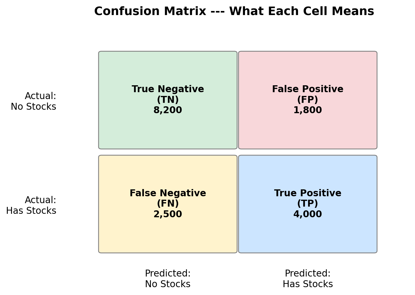
Visualise: Confusion Matrix
Reading the Confusion Matrix
Part 4
Evaluation Deep Dive
Why Accuracy is Not Enough
Imagine a dataset where 90% of people do NOT hold stocks.
A model that always predicts “No Stocks” gets 90% accuracy!
But it is completely useless — it never identifies a stock holder.
We need more nuanced metrics that look at different types of errors.
Four Fundamental Metrics
From the confusion matrix:
| Metric | Formula | Question It Answers |
|---|---|---|
| Sensitivity (Recall) | TP / (TP + FN) | Of all actual stock holders, how many did we find? |
| Specificity | TN / (TN + FP) | Of all non-holders, how many did we correctly identify? |
| Precision | TP / (TP + FP) | Of those we predicted as holders, how many actually are? |
| Accuracy | (TP + TN) / All | Overall, what fraction did we get right? |
Sensitivity vs Specificity
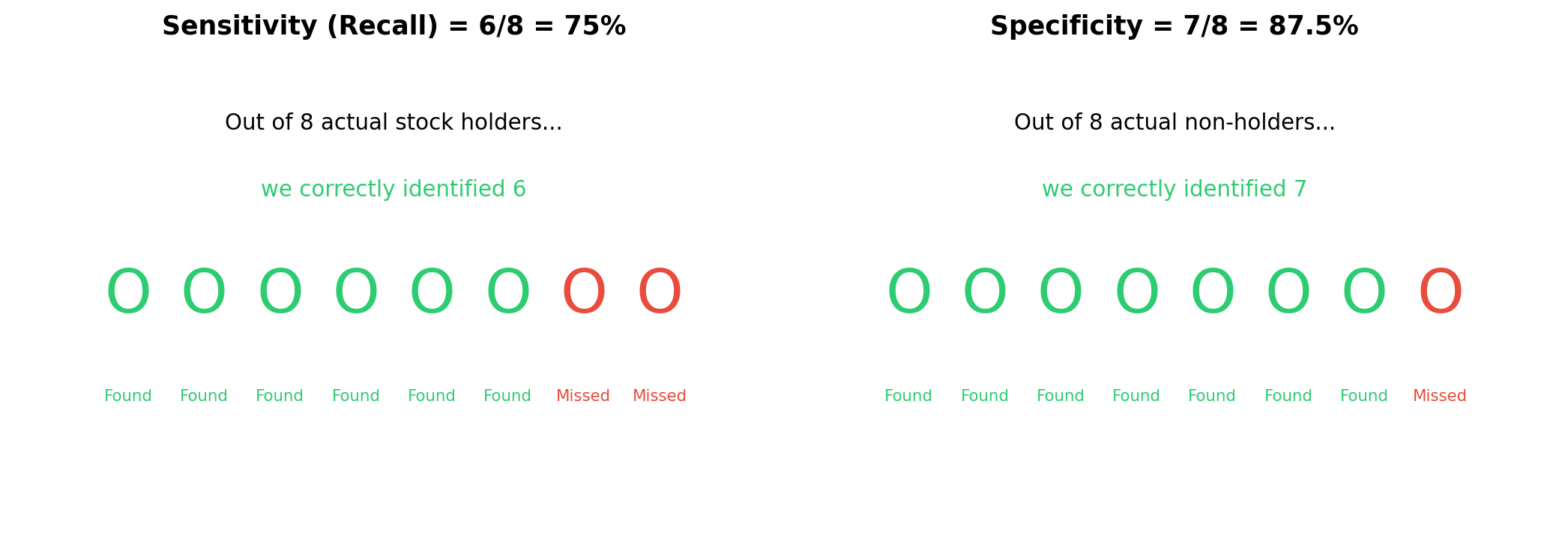
- Sensitivity: how good are we at finding stock holders?
- Specificity: how good are we at finding non-holders?
The Threshold Tradeoff
Logistic regression outputs a probability (0 to 1).
We choose a threshold to convert it to a prediction:
- Threshold = 0.5 (default): predict “Has Stocks” if probability > 50%
- Threshold = 0.3: more aggressive — catches more holders, but more false alarms
- Threshold = 0.7: more conservative — fewer false alarms, but misses more holders
There is always a tradeoff. Catching more positives = more false positives.
Visualising the Tradeoff
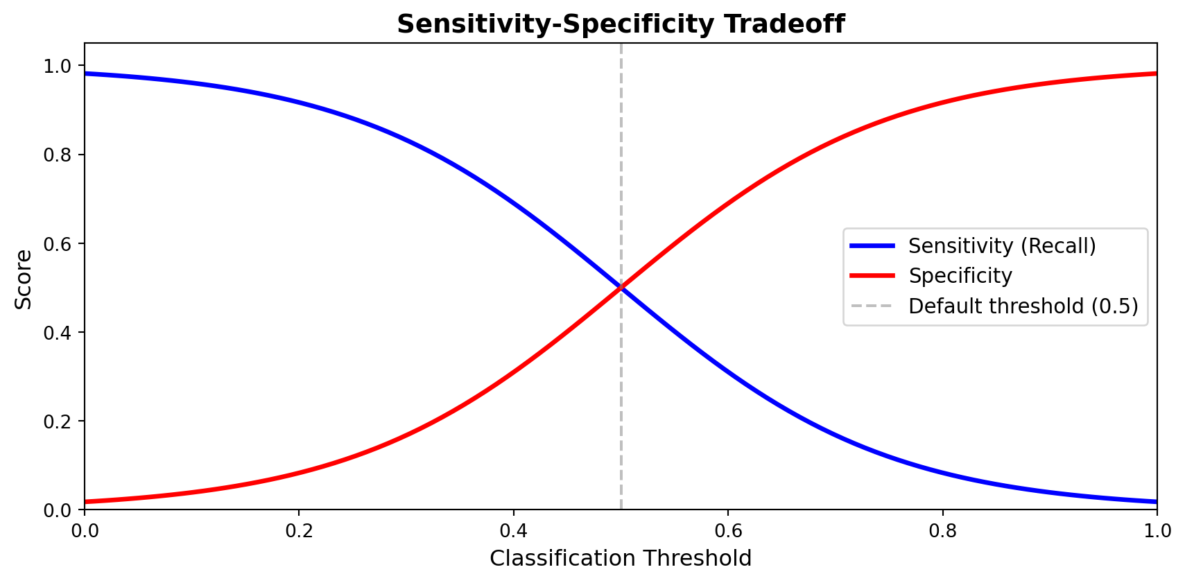
Lower the threshold → higher sensitivity, lower specificity.
ROC Curve
The ROC curve plots sensitivity vs (1 - specificity) at every threshold.
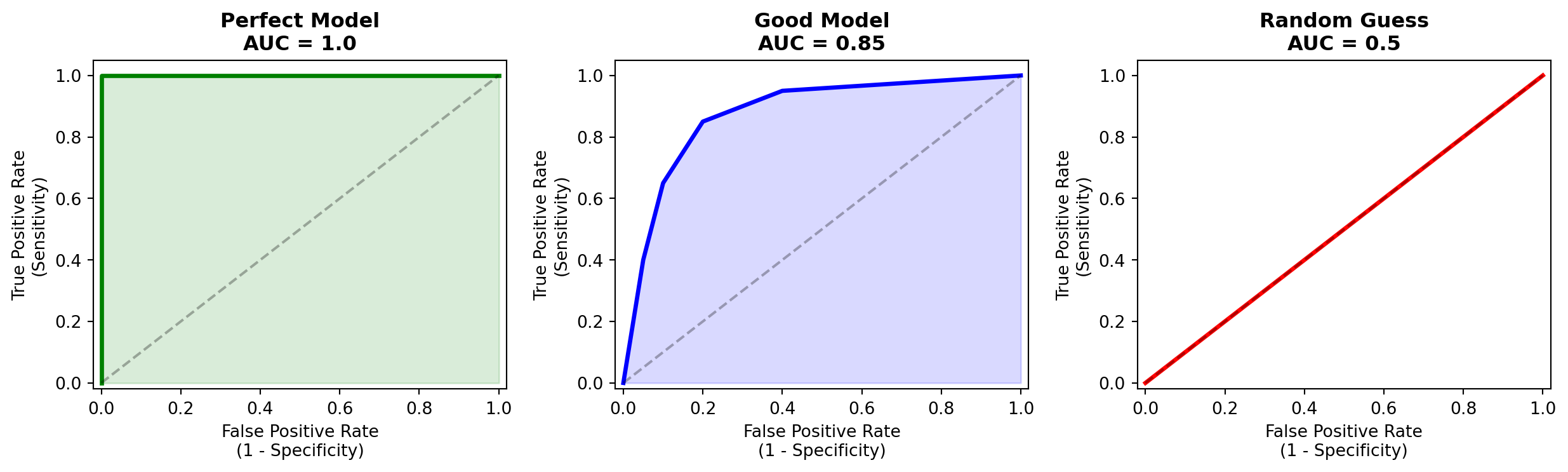
AUC (Area Under the Curve): one number summarising overall quality. Higher = better.
Precision vs Recall
| Metric | Focus | Use When… |
|---|---|---|
| Precision | Of predicted positives, how many are correct? | False positives are costly |
| Recall (= Sensitivity) | Of actual positives, how many did we find? | Missing positives is costly |
Stock participation example:
- High precision needed: acting on predictions costs money (targeted marketing)
- High recall needed: missing a stock holder means missing important data
F1 Score
When you care about both precision and recall:
\[F_1 = 2 \times \frac{\text{Precision} \times \text{Recall}}{\text{Precision} + \text{Recall}}\]
- F1 = 1.0: perfect precision and recall
- F1 = 0.0: either precision or recall is zero
- F1 penalises models that sacrifice one for the other
Which Metric for Our Problem?
For predicting stock market participation:
- AUC is a good default — evaluates across all thresholds
- F1 if we need a single threshold prediction
- Recall if we want to make sure we find all participants
In research, we typically report multiple metrics and let the reader judge.
Computing ROC for Our Model
Code
# ROC curve for logistic regression
fig, ax = plt.subplots(figsize=(8, 6))
RocCurveDisplay.from_estimator(
    grid_lr, X_test, y_test,
    name='Logistic Regression',
    ax=ax, color='steelblue', linewidth=2
)
ax.plot([0, 1], [0, 1], 'k--', alpha=0.3, label='Random (AUC = 0.5)')
ax.set_title('ROC Curve --- Stock Market Participation', fontsize=14)
ax.legend(fontsize=11)
plt.tight_layout()
plt.show()
Part 5
Model Comparison
The Power of Pipelines
Remember our pipeline structure:
To try a new model, we only change one line.
Gradient Boosting
Code
# Gradient Boosting --- a powerful ensemble method
pipeline_gb = Pipeline([
    ('preprocessor', preprocessor),
    ('classifier', GradientBoostingClassifier(random_state=42))
])

param_grid_gb = {
    'classifier__n_estimators': [100, 200],
    'classifier__learning_rate': [0.05, 0.1],
    'classifier__max_depth': [3, 5]
}

grid_gb = GridSearchCV(
    pipeline_gb, param_grid_gb,
    cv=5, scoring='roc_auc', n_jobs=-1, verbose=1
)
grid_gb.fit(X_train, y_train)

print(f'Best CV AUC: {grid_gb.best_score_:.4f}')
print(f'Best params: {grid_gb.best_params_}')
Random Forest
Code
# Random Forest --- another ensemble method
pipeline_rf = Pipeline([
    ('preprocessor', preprocessor),
    ('classifier', RandomForestClassifier(random_state=42))
])

param_grid_rf = {
    'classifier__n_estimators': [100, 200],
    'classifier__max_depth': [5, 10, None],
    'classifier__min_samples_leaf': [1, 5]
}

grid_rf = GridSearchCV(
    pipeline_rf, param_grid_rf,
    cv=5, scoring='roc_auc', n_jobs=-1, verbose=1
)
grid_rf.fit(X_train, y_train)

print(f'Best CV AUC: {grid_rf.best_score_:.4f}')
The Swap Pattern
# The pattern: only the classifier changes
from sklearn.svm import SVC
from sklearn.neighbors import KNeighborsClassifier
from sklearn.neural_network import MLPClassifier

models = {
    'Logistic Regression': LogisticRegression(max_iter=1000),
    'Random Forest':       RandomForestClassifier(n_estimators=200),
    'Gradient Boosting':   GradientBoostingClassifier(n_estimators=200),
    'SVM':                 SVC(probability=True),
    'KNN':                 KNeighborsClassifier(),
    'Neural Network':      MLPClassifier(max_iter=500),
}

for name, model in models.items():
    pipe = Pipeline([('preprocessor', preprocessor), ('classifier', model)])
    scores = cross_val_score(pipe, X_train, y_train, cv=5, scoring='roc_auc')
    print(f'{name:25s}  AUC = {scores.mean():.4f} +/- {scores.std():.4f}')
Compare ROC Curves
Code
# Side-by-side ROC curves
fig, ax = plt.subplots(figsize=(9, 7))

colors = {'Logistic Regression': 'steelblue',
          'Gradient Boosting': 'darkgreen',
          'Random Forest': 'darkorange'}

for name, grid in [('Logistic Regression', grid_lr),
                   ('Gradient Boosting', grid_gb),
                   ('Random Forest', grid_rf)]:
    RocCurveDisplay.from_estimator(
        grid, X_test, y_test,
        name=name, ax=ax,
        color=colors[name], linewidth=2
    )

ax.plot([0, 1], [0, 1], 'k--', alpha=0.3)
ax.set_title('Model Comparison --- ROC Curves', fontsize=14)
ax.legend(fontsize=11, loc='lower right')
plt.tight_layout()
plt.show()
Summary Table
Code
# Build comparison table
results = []
for name, grid in [('Logistic Regression', grid_lr),
                   ('Gradient Boosting', grid_gb),
                   ('Random Forest', grid_rf)]:
    y_pred = grid.predict(X_test)
    y_proba = grid.predict_proba(X_test)[:, 1]
    fpr, tpr, _ = roc_curve(y_test, y_proba)
    results.append({
        'Model': name,
        'CV AUC': f'{grid.best_score_:.4f}',
        'Test AUC': f'{auc(fpr, tpr):.4f}',
        'Test Accuracy': f'{accuracy_score(y_test, y_pred):.4f}',
        'Test F1': f'{f1_score(y_test, y_pred):.4f}'
    })

pd.DataFrame(results).set_index('Model')
Bias-Variance Tradeoff (Intuition)
Simple models (Logistic Regression)
- High bias, low variance
- Stable predictions
- May miss complex patterns
- Easy to interpret
Complex models (Gradient Boosting)
- Low bias, high variance
- Can capture subtle patterns
- Risk of overfitting
- Harder to interpret
No single model is always best. Compare fairly on test data and choose based on your goals.
Part 6
SHAP: Understanding Predictions
The Black Box Problem
We have a model that predicts stock participation with good AUC.
But why does it predict what it predicts?
- Which features matter most?
- How does each feature push the prediction up or down?
- Are the patterns economically sensible?
SHAP (SHapley Additive exPlanations) answers these questions.
What Are SHAP Values?
For each prediction, SHAP tells you:
How much did each feature contribute to this particular prediction?
Based on Shapley values from cooperative game theory:
- Each feature is a “player” in a game
- The “payout” is the prediction
- SHAP fairly distributes credit among features
Computing SHAP Values
Code
import shap

# Use the best model (e.g., Gradient Boosting)
best_model = grid_gb.best_estimator_

# Get the preprocessed test data
X_test_processed = best_model.named_steps['preprocessor'].transform(X_test)

# Get feature names after one-hot encoding
feature_names = (numerical_features +
    list(best_model.named_steps['preprocessor']
         .named_transformers_['cat']
         .named_steps['encoder']
         .get_feature_names_out(categorical_features)))

# Compute SHAP values
explainer = shap.TreeExplainer(best_model.named_steps['classifier'])
shap_values = explainer.shap_values(X_test_processed)
SHAP Summary Plot
How to read this plot:
- Features ranked by importance (top = most important)
- Each dot = one observation
- Red = high feature value, Blue = low
- Right of center = pushes prediction toward “Has Stocks”
Interpreting the Results
Expected patterns (from economic theory):
| Feature | Expected Effect | Why |
|---|---|---|
| Net Worth ↑ | More likely to hold stocks | Wealth enables risk-taking |
| Income ↑ | More likely | More to invest |
| Education (College+) | More likely | Financial literacy |
| Risk Aversion (high) | Less likely | Unwilling to bear risk |
| Age | Hump-shaped? | Lifecycle savings |
This is where ML meets economics: the model’s learned patterns should align with theory. If they don’t — that’s even more interesting.
SHAP for Individual Predictions
The waterfall plot shows:
- Starting from the base rate (average prediction)
- Each feature pushes the prediction up or down
- The final prediction is the sum of all contributions
Why SHAP Matters for Research
- Validation: Do the model’s patterns match economic theory?
- Discovery: Are there unexpected patterns we should investigate?
- Communication: Explain complex models to non-technical audiences
- Fairness: Check if the model relies on problematic features
ML is not just about getting a high AUC.
It’s about learning something useful from the data.
Wrap-Up
Summary
What We Covered Today
1. Why ML?          --> Prediction from data, different from causal inference
2. The Process      --> Split --> Preprocess --> Train --> Evaluate --> Compare
3. Live Demo        --> Complete pipeline with SCF data
4. Evaluation       --> Confusion matrix, ROC/AUC, precision/recall, F1
5. Model Comparison --> Swap algorithms in one line with Pipeline
6. SHAP             --> Open the black box, connect to economic theory
The Three Big Ideas
1. Process over algorithms
The workflow is the same for any model. Master the process.
2. Pipelines prevent mistakes
Preprocessing + model in one object. No data leakage. Easy to swap.
3. Prediction is just the beginning
SHAP and interpretability connect ML back to understanding — which is the real goal of research.
For Your Own Projects
# The template you can reuse for any classification problem:

# 1. Load and explore data
# 2. Define X (features) and y (target)
# 3. Train-test split with stratify
# 4. Build preprocessing pipeline
# 5. Build full pipeline (preprocessor + model)
# 6. GridSearchCV for hyperparameter tuning
# 7. Evaluate on test set
# 8. Try other models (just swap the classifier)
# 9. Compare with ROC curves
# 10. Interpret with SHAP
Resources
- scikit-learn documentation: scikit-learn.org
- SHAP documentation: shap.readthedocs.io
- This lecture’s code: available on the course GitHub